Revista Colombiana de
Tecnologías de Avanzada
Tecnologías de Avanzada
Recibido: 04 de abril de 2023
Aceptado: 10 de julio de 2023
Aceptado: 10 de julio de 2023
ESTUDIO HIDRODINÁMICO DE UN REACTOR ANULAR DE FASE LÍQUIDA Y AGITADO CON AIRE
HYDRODYNAMIC STUDY OF AN ANNULAR LIQUID PHASE/AIR STIRRED REACTOR
MSc. Daniela Montaño-Bello*, PhD. Hugo Ricardo Zea Ramírez*
* Universidad Nacional de Colombia, Facultad de Ingeniería, Sede Bogotá.
Carrera 30 no 45 – 03, Bogotá Colombia.
Tel.: 57+1+3165000 ext. 14303.
E-mail: {dmontanob, hrzear}@unal.edu.co
https://orcid.org/0000-0003-4793-898X
https://orcid.org/0000-0002-6801-1879
Cómo citar: Montaño-Bello, D., & Zea Ramírez, H. R. (2023). ESTUDIO HIDRODINÁMICO DE UN REACTOR ANULAR DE FASE LÍQUIDA Y AGITADO CON AIRE. REVISTA COLOMBIANA DE TECNOLOGIAS DE AVANZADA (RCTA), 2(42), 7–16. https://doi.org/10.24054/rcta.v2i42.2648
Derechos de autor 2023 Revista Colombiana de Tecnologías de Avanzada (RCTA).
Esta obra está bajo una licencia internacional Creative Commons Atribución-NoComercial 4.0.

Esta obra está bajo una licencia internacional Creative Commons Atribución-NoComercial 4.0.
Resumen: La caracterización hidrodinámica de reactores químicos es un paso clave en el diseño de plantas piloto y reactores a escala industrial. En este trabajo se determinó la distribución del tiempo de residencia y el modelo de flujo para un reactor anular multifásico de 12 litros. Utilizando experimentos de entrada de pulsos, se determinó la distribución del tiempo de residencia (RTD) de acuerdo con las variaciones de los parámetros de flujo, empacado y agitación. Comparando la respuesta del trazador con los modelos de flujo, el modelo de tanques agitados en serie con n=4 se ajusta mejor al reactor sin agitación, mientras que el modelo CSTR es mejor para la configuración de un reactor agitado con aire.
Palabras clave: Hidrodinámica, distribución del tiempo de residencia RTD, dispersión, reactor CSTR.
Abstract: Chemical reactors hydrodynamic characterization is a key step in the design of pilot plant and industrial scale reactors. In this work, the residence time distribution and the flow model were determined for a 12 liters annular multiphase reactor. Using pulse input experiments, the residence time distribution (RTD) was determined according to parameters variations of flow, packaging and stirring. Comparing tracer response with the flow models, stirred tanks in series model with n=4 fits the best for the reactor without agitation while the CSTR model is the better for the configuration of an air stirred reactor.
Keywords: Hydrodynamic, residence time distribution RTD, dispersion, CSTR reactor.
Before any reaction experiment take place, it is important to know the flow patter distribution of the vessel in which the reaction will take place. A significant challenge to develop industrial application is to scale the benchtop experiments to pilot plant and industrial scale setting
2.1 Pulse input experiment
For the hydrodynamic study, a solution of Orange II dye is used. By a pulse input experiment, 60 ml of a solution with a concentration 2 g/L of Orange II dye are injected, and then the reactor output concentration is measured over time. The dye concentration at the outlet is determined by measuring the absorbance of the samples collected using a spectrophotometer, for that purpose a calibration curve is previously performed. For a pulse input experiment, the E(t) curve is given by the following equation, where C(t) refers to the tracer outlet response
\[ E(t) = \frac{C(t)}{\int_{0}^{\infty} C(t) \, dt} \hspace{1cm} (1)\] Besides, the accumulative distribution function F(t) is built to know the fraction of effluent that has been in the reactor less than the time t
\[ \int_{0}^{t} E(t) \, dt = F(t) \hspace{1cm} (2)\] As well, the fraction of effluent that has been in the reactor for a time higher than t
\[ \int_{t}^{\infty} E(t) \, dt = 1 - F(t) \hspace{1cm} (3)\]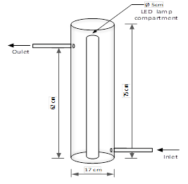
To study the effect of the parameters on the annular catalytic reactor, a 2k factorial design is used to see if there are any added effects of the parameters. The hydrodynamic behavior involves 3 factors, which are flow, packaging and stirring. At 2 levels requires 2 × 2 × 2 = 8 experiments [9] to obtain all possible combinations. By measuring the output concentration over a given time, the tracer concentration curve is obtained to determine the residence time distribution (RTD). The curves E(t), F(t) y 1-F(t) and the dimensionless distribution function E(θ) were constructed. In addition, the RTD moments like mean residence time and variance were calculated. The integrals of the different equations have been made by numerical integration of the Simpsons rule of 1/3 and 3/8 according to the selected interval. Dimensionless distribution function E(θ) is used to determine the reactor flow model compared to dispersion, stirred tanks in series and CSTR models.
In the reactor was observed that once the dye tracer was injected, the streamlines flow radially towards the facing wall of the inner cylinder and finally surrounds it. This behavior has also been described in CFD simulation articles where the jet separation around the radial flow path of the streamline introduces a flapping motion, making the flow perpendicular to the main reactor axis
Observing to Figure 3-a, even though the flow rate for the first test E1 is much less compared to the E2 and E3 tests, the distribution curves have a similar behavior. In the E(t) curve, it is observed that the dye started to come out after almost two and a half minutes after the injection. This delay means that within the reactor there is a combine effect of plug flow in series with stirred tank flow (Levenspiel, n.d.). Also, the stepped behavior indicates a slow internal circulation suggesting inadequate mixing
The accumulative distribution (see Fig. 4b) for test 2 and 3 it reaches 10 min, so all the dye leaves the reactor after 10 min. In general, 80% of the dye remained less than 6 minutes in the reactor.
The accumulative distribution for test 1 and 2, 60% of the dye pass between 3.5 and 5 minutes inside the reactor. Whereas for test 1, the 60% of the particles remained less than 2 minutes in the reactor. Also, there is a shift to the left on the F (t) curve for test 3, the change in shape of this curve predicts reactor flow problems such as short circuits.
After characterizing the behavior of the flow inside the reactor for the different experiments and determining the possible hydraulic problems as the short circuits and the dead zones, an assessment to compare the results obtained experimentally against reactors mathematical model was performed.
In the stirred tanks in series model, the E(t) curve for n tanks is
\[ E(t) = \frac{t^{n-1}}{(n-1)! \tau_i^n} \cdot e^{-\frac{t}{\tau_i}} \hspace{1cm} (4)\] For the construction of the dimensionless E(ϴ) curve, where ϴ=t/τ and τi=τ/n then the equations become
\[ E(\theta) = \frac{{n (n\theta)^{n-1}}}{{(n-1)!}} \cdot e^{-n\theta} \hspace{1cm} (5)\] In the dispersion model, the E(ϴ) curve is constructed by the equation [12]:
\[ E(\theta) = \frac{1}{{2\sqrt{\pi \theta \left(\frac{D}{uL}\right)}}} \cdot e^{-\frac{(1-\theta)^2}{4 \theta \left(\frac{D}{uL}\right)}} \hspace{1cm} (6)\] This dimensionless term (D/uL) can be grouped into a non-dimensional term known as the Peclet number of reactor (\({Pe}_r\)):
\[ \text{Pe}_r = \frac{uL}{D} \hspace{1cm} (7)\] Where L refers to the length of the reactor, u is the velocity of the fluid. When the dispersion is negligible (D/uL) this term tends to zero and therefore Per tends to infinity, then behaves more like a piston flow. If Per tends to zero is because the dispersion is large (D / uL) tends to infinity and is closer to a complete mixture flow
\[ \frac{D}{uL} \to 0 \quad \text{ } \quad \text{Pe}_r \to \infty \quad \text{tends to PFR} \] \[ \frac{D}{uL} \to 0 \quad \text{ } \quad \text{Pe}_r \to \infty \quad \text{tends to CSTR} \] When the residence time distribution is asymmetric, the dispersion may be large
In general, for all the experiments performed by varying the flow and packaging in the reactor without stirring, the model that best fits the experimental data is the model of tanks in series with four tanks (n = 4).
The experiment with minimum flow and packaging has the lowest correlation with the dispersion model (see table 2). It can be noticed that the dispersion model fits the long tail of the E (ϴ) curve but does not adjust to the maximum.
Residence time distribution (RTD), mean residence time and variance were evaluated for each test of the experiments without stirring according to the following equations. The mean time (\(t_m\)) is given by
\[ t_m = \frac{\int_{0}^{\infty} t \, E(t) \, dt}{\int_{0}^{\infty} E(t) \, dt} = \int_{0}^{\infty} t \, E(t) \, dt \hspace{1cm} (9)\] The variance (\(\sigma^2\)) is given by
\[ \sigma^2 = \int_{0}^{\infty} (t - t_m)^2 \, E(t) \, dt \hspace{1cm} (10)\] Table 3 shows the mean retention time of the experiments and their repetitions, the experiment minimum flow and without packaging has the highest mean time. Comparing the minimum flow experiments, the ones with the mesh have shorter residence times compared to experiments without packaging. Therefore, in low flow operation the packaging should be consider as a parameter directly affecting the residence time in the 12 liters annular catalytic reactor. In a certain way, the mesh changes the movement of the particles into the reactor when working at low flow rates.
On the other hand, in a comparison between the experiments with maximum flow, the residence times are very close except for the third test with a mean time of 1.9 minutes. Where it may be caused because of a short circuit or bypass that allowed the tracer coming out much faster than in the other test of the same experiment. Consequently, the effect of the mesh for low flows is not the same for high flows.
In Table 4, the variance for each test of the four experiments is shown; the highest variances belong to the minimum flux experiments. The magnitude of the variance is an indication of the dispersion of the distribution
In general, the values of variance differ significantly from test to test of the same experiment, especially for those experiments with minimum flow. This is due to the difference in the response curves of the tests in the same experiment as discussed previously.
Furthermore, the accumulative distribution (see Figure 10-b), the 60% of the dye remained less than 5 minutes in the reactor. After the injection of the dye, the flow inside the reactor acquired the same orange coloration in a few seconds (less than 20 seconds). The intensity of color decreased gradually over the time.
In a comparison of dye behavior inside the reactor between the experiments without stirring and the experiments with air stirring, is observed that in the ones without stirring takes several minutes to color all the fluid homogenously, since for air stirred experiments takes only few seconds. In addition, at the end when the last colorant comes out, for the non-stirring experiments the bottom became transparent and more orange at the top in a degrade scale, so different to the behavior of the reactor with air stirring that have the same color tone along the reactor.
According to the Figure 8-a, the E(t) curves had also a decreasing behavior expect for the first point. As is shown on Figure 8-b, the accumulative distribution F(t) curve the 60% of the dye remained less than 7 minutes and more than 4 minutes inside the reactor.
According to the accumulative distribution F(t) in the Figure 9-b, the 80% of the particles remained between 1 minute to 6 minutes inside the reactor.
\[ E(t) = \frac{e^{-\frac{t}{\tau}}}{\tau} \hspace{1cm} (11)\] Remembering that ϴ=t/τ and E(ϴ)= τE(t) [9], then
\[ E(\theta) = e^{-\theta} \hspace{1cm} (12)\] All the experiments have a similar behavior to an ideal CSTR reactor model, but only the experiment with the packaging mesh and maximum flow starts in 1 as the model CSTR do it. In general, the experiments with the packaging mesh have the best correlation coefficient with CSTR (see table 5).
In other studies of RTD in stirred annular reactors, they also have observed in gas phase with a magnetic stirrer that a higher stirring rate broadened the RTD curve drastically and the reactor increasingly behaved as a single stirred tank reactor (Sahle-Demessie et al., 2003). Comparing a magnetic stirrer and airlift stirring, the first ones need higher velocities to produce a significant change in the RTD curve, while the second one stirs the entire flow along the reactor.
Residence time distribution (RTD) as mean residence time and variance were also evaluated, according to the equations 9 and 10. For the air stirred experiments, the minimum mean residence time corresponds to the experiment with the packaging mesh with a maximum flow operation (see table 6). Also, the lower value of variance corresponds to this experiment.
A comparison between the experiments without the mesh, a change in the airflow does not create a big impact in mean time observed. Hence, even a minimum airflow for stirring will make a good stirring of the fluid along the entire reactor.
In addition, it was determined that the residence time in the reactor without stirring comes from 4 to 10 minutes and for airlift reactor the residence time comes from 3.5 to 6.6 minutes, depending on the flow and packaging operation conditions
The analysis of the residence time distribution allowed to validate the model that best predicts the behavior of the 12-liters annular reactor without agitation. Stirred tanks in series model with n=4 fits the best for the reactor without agitation while the CSTR model is the better for the configuration of airlift reactor.
Ekambara, K., Dhotre, M. T., & Joshi, J. B. (2006). CFD simulation of homogeneous reactions in turbulent pipe flows—Tubular non-catalytic reactors. Chemical Engineering Journal, 117(1), 23–29. https://doi.org/https://doi.org/10.1016/j.cej.2005.12.006
Fogler, H. S. (n.d.). Elements of chemical reaction engineering. Third edition. Upper Saddle River, N.J. : Prentice Hall PTR, [1999] ©1999. https://search.library.wisc.edu/catalog/999810177702121
Hissanaga, A. M., Padoin, N., & Paladino, E. E. (2020). Mass transfer modeling and simulation of a transient homogeneous bubbly flow in a bubble column. Chemical Engineering Science, 218, 115531. https://doi.org/https://doi.org/10.1016/j.ces.2020.115531
Levenspiel, O. (n.d.). Chemical reaction engineering. Third edition. New York : Wiley, [1999] ©1999. https://search.library.wisc.edu/catalog/999917971402121
Sahle-Demessie, E., Bekele, S., & Pillai, U. R. (2003). Residence time distribution of fluids in stirred annular photoreactor. Catalysis Today, 88(1), 61–72. https://doi.org/https://doi.org/10.1016/j.cattod.2003.08.009
Sangare, D., Bostyn, S., Moscosa-Santillan, M., & Gökalp, I. (2021). Hydrodynamics, heat transfer and kinetics reaction of CFD modeling of a batch stirred reactor under hydrothermal carbonization conditions. Energy, 219, 119635. https://doi.org/https://doi.org/10.1016/j.energy.2020.119635
Shu, S., Vidal, D., Bertrand, F., & Chaouki, J. (2019). Multiscale multiphase phenomena in bubble column reactors: A review. Renewable Energy, 141, 613–631. https://doi.org/https://doi.org/10.1016/j.renene.2019.04.020
Sozzi, D. A., & Taghipour, F. (2006). Computational and experimental study of annular photo-reactor hydrodynamics. International Journal of Heat and Fluid Flow, 27(6), 1043–1053. https://doi.org/https://doi.org/10.1016/j.ijheatfluidflow.2006.01.006
Vandewalle, L. A., Van de Vijver, R., Van Geem, K. M., & Marin, G. B. (2019). The role of mass and heat transfer in the design of novel reactors for oxidative coupling of methane. Chemical Engineering Science, 198, 268–289. https://doi.org/https://doi.org/10.1016/j.ces.2018.09.022
Palabras clave: Hidrodinámica, distribución del tiempo de residencia RTD, dispersión, reactor CSTR.
Abstract: Chemical reactors hydrodynamic characterization is a key step in the design of pilot plant and industrial scale reactors. In this work, the residence time distribution and the flow model were determined for a 12 liters annular multiphase reactor. Using pulse input experiments, the residence time distribution (RTD) was determined according to parameters variations of flow, packaging and stirring. Comparing tracer response with the flow models, stirred tanks in series model with n=4 fits the best for the reactor without agitation while the CSTR model is the better for the configuration of an air stirred reactor.
Keywords: Hydrodynamic, residence time distribution RTD, dispersion, CSTR reactor.
1. INTRODUCTION
Many factors interact in the design and operation of multiphase reactors: the reaction kinetic, the involved fluids hydrodynamic, the contact between the phases, the turbulence generated and, in general, the transport and surface phenomena(Sangare et al., 2021;
Sangare, D., Bostyn, S., Moscosa-Santillan, M., & Gökalp, I. (2021). Hydrodynamics, heat transfer and kinetics reaction of CFD modeling of a batch stirred reactor under hydrothermal carbonization conditions. Energy, 219, 119635. https://doi.org/https://doi.org/10.1016/j.energy.2020.119635
Vandewalle et al., 2019)
. In multiphase systems, the interaction of several phases implies that the rate of reaction is a strong function of the effectiveness of the phases contact. The complexity of hydrodynamics behavior fluctuates considerably on the ratio of the involved phases flow rates. Given the extensive variety of existing hydrodynamic models, it is not easy to choose one model that adequately describes the hydrodynamics of the reactive system without first experimentally recognizing the behavior of the proposed reactor design Vandewalle, L. A., Van de Vijver, R., Van Geem, K. M., & Marin, G. B. (2019). The role of mass and heat transfer in the design of novel reactors for oxidative coupling of methane. Chemical Engineering Science, 198, 268–289. https://doi.org/https://doi.org/10.1016/j.ces.2018.09.022
(Aparicio-Mauricio et al., 2017;
Aparicio-Mauricio, G., Ruiz, R. S., López-Isunza, F., & Castillo-Araiza, C. O. (2017). A simple approach to describe hydrodynamics and its effect on heat and mass transport in an industrial wall-cooled fixed bed catalytic reactor: ODH of ethane on a MoVNbTeO formulation. Chemical Engineering Journal, 321, 584–599. https://doi.org/https://doi.org/10.1016/j.cej.2017.03.043
Hissanaga et al., 2020;
Hissanaga, A. M., Padoin, N., & Paladino, E. E. (2020). Mass transfer modeling and simulation of a transient homogeneous bubbly flow in a bubble column. Chemical Engineering Science, 218, 115531. https://doi.org/https://doi.org/10.1016/j.ces.2020.115531
Shu et al., 2019)
. In chemical reaction kinetics, the controlling step is always the slowest, so the overall reaction rate is equal to the slowest stage. Then, if the mass transfer steps are controlling the rate, a change in flow or operation conditions can modify the global catalytic rate Shu, S., Vidal, D., Bertrand, F., & Chaouki, J. (2019). Multiscale multiphase phenomena in bubble column reactors: A review. Renewable Energy, 141, 613–631. https://doi.org/https://doi.org/10.1016/j.renene.2019.04.020
(Ekambara et al., 2006;
Ekambara, K., Dhotre, M. T., & Joshi, J. B. (2006). CFD simulation of homogeneous reactions in turbulent pipe flows—Tubular non-catalytic reactors. Chemical Engineering Journal, 117(1), 23–29. https://doi.org/https://doi.org/10.1016/j.cej.2005.12.006
Shu et al., 2019)
. Mass transfer can be a factor that influence the reaction rate, for this reason is important to know the hydrodynamic behavior in the reactor.Shu, S., Vidal, D., Bertrand, F., & Chaouki, J. (2019). Multiscale multiphase phenomena in bubble column reactors: A review. Renewable Energy, 141, 613–631. https://doi.org/https://doi.org/10.1016/j.renene.2019.04.020
Before any reaction experiment take place, it is important to know the flow patter distribution of the vessel in which the reaction will take place. A significant challenge to develop industrial application is to scale the benchtop experiments to pilot plant and industrial scale setting
(Levenspiel, 1999)
. In this study a detailed study of the hydrodynamic behavior of a 12-liter annular flow reactor along with a residence time distribution (RTD) analysis.Levenspiel, O. (n.d.). Chemical reaction engineering. Third edition. New York : Wiley, [1999] ©1999. https://search.library.wisc.edu/catalog/999917971402121
2. MATERIALS AND METHODS
The catalytic reactor under study has a vertical tubular shape and, in the center, has an annular cylinder used to enclose the set of LED lamps, in the case photocatalytic reactions want to be performed. The feed to the reactor is located on the bottom and the outlet is on the top. The reactor volume is 12 liters, continuously fed by a centrifugal pump. Figure 1 shows a schematic diagram of the annular catalytic reactor.2.1 Pulse input experiment
For the hydrodynamic study, a solution of Orange II dye is used. By a pulse input experiment, 60 ml of a solution with a concentration 2 g/L of Orange II dye are injected, and then the reactor output concentration is measured over time. The dye concentration at the outlet is determined by measuring the absorbance of the samples collected using a spectrophotometer, for that purpose a calibration curve is previously performed. For a pulse input experiment, the E(t) curve is given by the following equation, where C(t) refers to the tracer outlet response
(Fogler, n.d.)
.Fogler, H. S. (n.d.). Elements of chemical reaction engineering. Third edition. Upper Saddle River, N.J. : Prentice Hall PTR, [1999] ©1999. https://search.library.wisc.edu/catalog/999810177702121
\[ E(t) = \frac{C(t)}{\int_{0}^{\infty} C(t) \, dt} \hspace{1cm} (1)\] Besides, the accumulative distribution function F(t) is built to know the fraction of effluent that has been in the reactor less than the time t
(Fogler, n.d.)
:Fogler, H. S. (n.d.). Elements of chemical reaction engineering. Third edition. Upper Saddle River, N.J. : Prentice Hall PTR, [1999] ©1999. https://search.library.wisc.edu/catalog/999810177702121
\[ \int_{0}^{t} E(t) \, dt = F(t) \hspace{1cm} (2)\] As well, the fraction of effluent that has been in the reactor for a time higher than t
(Fogler, n.d.)
:Fogler, H. S. (n.d.). Elements of chemical reaction engineering. Third edition. Upper Saddle River, N.J. : Prentice Hall PTR, [1999] ©1999. https://search.library.wisc.edu/catalog/999810177702121
\[ \int_{t}^{\infty} E(t) \, dt = 1 - F(t) \hspace{1cm} (3)\]
Fig. 1. Schematic diagram of the annular catalytic reactor.
2.2 Experimental factorial designTo study the effect of the parameters on the annular catalytic reactor, a 2k factorial design is used to see if there are any added effects of the parameters. The hydrodynamic behavior involves 3 factors, which are flow, packaging and stirring. At 2 levels requires 2 × 2 × 2 = 8 experiments [9] to obtain all possible combinations. By measuring the output concentration over a given time, the tracer concentration curve is obtained to determine the residence time distribution (RTD). The curves E(t), F(t) y 1-F(t) and the dimensionless distribution function E(θ) were constructed. In addition, the RTD moments like mean residence time and variance were calculated. The integrals of the different equations have been made by numerical integration of the Simpsons rule of 1/3 and 3/8 according to the selected interval. Dimensionless distribution function E(θ) is used to determine the reactor flow model compared to dispersion, stirred tanks in series and CSTR models.
3. RESULT AND DISCUSSION
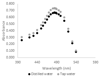
Since the catalytic reactor is operated with tap water, there must not be interference from the other components present in the tap water (such as iron that is came from old pipes), in the detection of the maximum absorbance of the Orange II dye. For this purpose, a comparison between dye solutions with distilled water and with tap water was made to see if the detection maximum of the curve for Orange II was the same in both cases. Figure 2 shows the absorbance curve of distilled water and tap water (both with a concentration of 30.9 mg/L) at different wavelengths. For all wavelengths, tap water solutions had higher absorbance values than distillated water solutions. However, the maximum point in both cases was at 484nm. The same test was also performed for solutions with a concentration of 25.6 mg/L, obtaining the same result as the maximum absorbance at 484 nm.
Fig. 2. Absorbance at different wavelengths for dye solutions (Orange II), with distilled water and tap water.
3.1 Experiments without stirring
3.1.1 Minimum flow, without packaging.
The experiment was performed with the inlet valve half open, the reactor without the packaging mesh and without stirring. The flow rates for the three tests are: 11.94 ml / s for test 1, for test 2 it is 18.50 ml / s and for test 3 is 18.32 ml / s.In the reactor was observed that once the dye tracer was injected, the streamlines flow radially towards the facing wall of the inner cylinder and finally surrounds it. This behavior has also been described in CFD simulation articles where the jet separation around the radial flow path of the streamline introduces a flapping motion, making the flow perpendicular to the main reactor axis
(Sozzi & Taghipour, 2006)
. Sozzi, D. A., & Taghipour, F. (2006). Computational and experimental study of annular photo-reactor hydrodynamics. International Journal of Heat and Fluid Flow, 27(6), 1043–1053. https://doi.org/https://doi.org/10.1016/j.ijheatfluidflow.2006.01.006
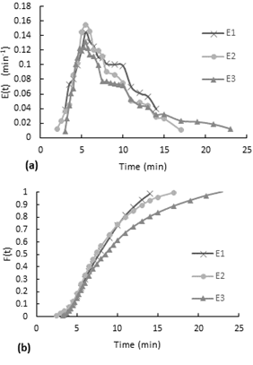
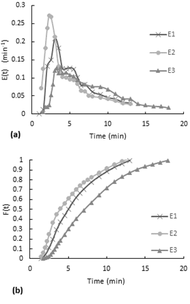
Observing to Figure 3-a, even though the flow rate for the first test E1 is much less compared to the E2 and E3 tests, the distribution curves have a similar behavior. In the E(t) curve, it is observed that the dye started to come out after almost two and a half minutes after the injection. This delay means that within the reactor there is a combine effect of plug flow in series with stirred tank flow (Levenspiel, n.d.). Also, the stepped behavior indicates a slow internal circulation suggesting inadequate mixing
(Levenspiel, n.d.)
.Levenspiel, O. (n.d.). Chemical reaction engineering. Third edition. New York : Wiley, [1999] ©1999. https://search.library.wisc.edu/catalog/999917971402121
Fig. 3. Residence time distribution curves for the minimum flow, no packaging, and no stirring experiment.
(a) E(t) curve, (b) accumulative distribution function F(t).
Moreover, the accumulative distribution (see Figure 3b), for the three tests the 60% of the dye remained 6.5 to 10 minutes in the reactor.(a) E(t) curve, (b) accumulative distribution function F(t).
3.1.2 Maximum flow, without packaging.
The experiment was performed with the inlet valve fully open, the reactor without the packaging mesh and without stirring. The average flow rate is 40.46 ml/s.The accumulative distribution (see Fig. 4b) for test 2 and 3 it reaches 10 min, so all the dye leaves the reactor after 10 min. In general, 80% of the dye remained less than 6 minutes in the reactor.
Fig. 4. Residence time distribution curves for the maximum flow, no packaging, and no stirring experiment.
(a) E(t) curve, (b) accumulative distribution function F(t).
In the pulse input experiment, the tracer started to come out the reactor after one minute of the dye injection (See Figure 4-a). This delay means that in the reactor behaves like a plug flow in series with mixed flow as in the minimum flow experiment. The delay time is half the delay time of the previous experiment that was performed using a lower flow rate.(a) E(t) curve, (b) accumulative distribution function F(t).
3.1.3 Minimum flow, with packaging.
The experiment was performed with the inlet valve half open, the reactor with the packaging mesh and without stirring. The average flow rates for the 3 tests are 18.85ml/s for test 1, for test 2 it is 17.65ml/s and for test 3 it is 21.98ml/s.
Fig. 5. Residence time distribution curves for the minimum flow, with packaging and no stirring experiment.
(a) C(t) curve, (b) accumulative distribution function F(t).
In the E(t) curve, is observed that the dye started to come out one and a half minutes after the injection (see Figure 5-a), it is also observed that the test 2 presents a different behavior than the other tests, obtaining a significantly higher maximum compared to test 1 and 3. In all three tests used the same concentration of dye and the same injection volume, therefore the behavior of test 2 is strange. Although it has the lowest flow rate of the three tests, the colorant exits much faster. On the other hand, the double maximum of the curve C (t) for test 3 indicates that there are parallel paths (a) C(t) curve, (b) accumulative distribution function F(t).
(Levenspiel, n.d.)
. There may exist stagnant waters or dead zone. The accumulative distribution is simulated for trials 2 and 3 (see Figure 5-b). If E1 is compared to E3, in the first 80% of the dye remain between 3 and 9 minutes in the reactor, in the second 80% of the particles pass between 4 and 12 minutes inside the reactor.Levenspiel, O. (n.d.). Chemical reaction engineering. Third edition. New York : Wiley, [1999] ©1999. https://search.library.wisc.edu/catalog/999917971402121
3.1.4 Maximum flow, with packaging.
The experiment was performed with the inlet valve fully open, the reactor with the packaging mesh and without stirring. In Figure 6, the sequence of the dye behavior within the reactor is observed. At the beginning, a concentrated solution is injected, which is diluted as it ascends through the reactor, and in this ascent, it is possible to see a kind of swirl that does not completely cover all the zones. After a few minutes, much of the dye has left the reactor and the remainder is distributed in a particular way, the lower part turns transparent, and the intensity of the dye increases gradually upwards toward the reactor outlet. This same color gradient behavior was observed in all experiments without agitation.The accumulative distribution for test 1 and 2, 60% of the dye pass between 3.5 and 5 minutes inside the reactor. Whereas for test 1, the 60% of the particles remained less than 2 minutes in the reactor. Also, there is a shift to the left on the F (t) curve for test 3, the change in shape of this curve predicts reactor flow problems such as short circuits.
Fig. 6. Residence time distribution curves for the maximum flow, with packaging and no stirring experiment.
(a) E(t) curve, (b) accumulative distribution function F(t)
According to results, is observed that the test E3 has a different behavior than the tests E1 and E2 although having the same concentration of dye and the same volume of injection. As in experiment with minimum flow and packaging, one of the tests has a much higher maximum than the rest tests. Also, the dye started to come out after one minute for tests E1 and E2. In contrast, for test E3 the response was almost instantaneous, the first sample was collected after 15 seconds because the rapid coming out of the dye. In this case, the behavior of test 3 may be explained by short-circuited flow path in the reactor since the output time is almost instantaneous. (a) E(t) curve, (b) accumulative distribution function F(t)
After characterizing the behavior of the flow inside the reactor for the different experiments and determining the possible hydraulic problems as the short circuits and the dead zones, an assessment to compare the results obtained experimentally against reactors mathematical model was performed.
In the stirred tanks in series model, the E(t) curve for n tanks is
(Fogler, n.d.)
:Fogler, H. S. (n.d.). Elements of chemical reaction engineering. Third edition. Upper Saddle River, N.J. : Prentice Hall PTR, [1999] ©1999. https://search.library.wisc.edu/catalog/999810177702121
\[ E(t) = \frac{t^{n-1}}{(n-1)! \tau_i^n} \cdot e^{-\frac{t}{\tau_i}} \hspace{1cm} (4)\] For the construction of the dimensionless E(ϴ) curve, where ϴ=t/τ and τi=τ/n then the equations become
(Fogler, n.d.;
Fogler, H. S. (n.d.). Elements of chemical reaction engineering. Third edition. Upper Saddle River, N.J. : Prentice Hall PTR, [1999] ©1999. https://search.library.wisc.edu/catalog/999810177702121
Levenspiel, n.d.)
,Levenspiel, O. (n.d.). Chemical reaction engineering. Third edition. New York : Wiley, [1999] ©1999. https://search.library.wisc.edu/catalog/999917971402121
\[ E(\theta) = \frac{{n (n\theta)^{n-1}}}{{(n-1)!}} \cdot e^{-n\theta} \hspace{1cm} (5)\] In the dispersion model, the E(ϴ) curve is constructed by the equation [12]:
\[ E(\theta) = \frac{1}{{2\sqrt{\pi \theta \left(\frac{D}{uL}\right)}}} \cdot e^{-\frac{(1-\theta)^2}{4 \theta \left(\frac{D}{uL}\right)}} \hspace{1cm} (6)\] This dimensionless term (D/uL) can be grouped into a non-dimensional term known as the Peclet number of reactor (\({Pe}_r\)):
\[ \text{Pe}_r = \frac{uL}{D} \hspace{1cm} (7)\] Where L refers to the length of the reactor, u is the velocity of the fluid. When the dispersion is negligible (D/uL) this term tends to zero and therefore Per tends to infinity, then behaves more like a piston flow. If Per tends to zero is because the dispersion is large (D / uL) tends to infinity and is closer to a complete mixture flow
(Levenspiel, n.d.)
.Levenspiel, O. (n.d.). Chemical reaction engineering. Third edition. New York : Wiley, [1999] ©1999. https://search.library.wisc.edu/catalog/999917971402121
\[ \frac{D}{uL} \to 0 \quad \text{ } \quad \text{Pe}_r \to \infty \quad \text{tends to PFR} \] \[ \frac{D}{uL} \to 0 \quad \text{ } \quad \text{Pe}_r \to \infty \quad \text{tends to CSTR} \] When the residence time distribution is asymmetric, the dispersion may be large
(Levenspiel, n.d.)
. Then the variance \(\sigma_{\theta}^2\) is given by:
\[ \sigma_{\theta}^2 = \frac{\sigma^2}{\tau^2} = 2\left(\frac{D}{uL}\right) - 2\left(\frac{D}{uL}\right)^2 (1 - e^{-uL/D}) \hspace{0.4cm} (8)\]
For the dispersion model is necessary to know the value of the variance (\(\sigma_{\theta}^2\)), to calculate the dimensionless number of Peclet and then obtain the value of E(ϴ), by equations 6 and 8. In the table I, the parameters for the calculation of the dispersion model are shown.Levenspiel, O. (n.d.). Chemical reaction engineering. Third edition. New York : Wiley, [1999] ©1999. https://search.library.wisc.edu/catalog/999917971402121
Table 1: Parameters calculated for the dispersion model.
| Experiment | \(\sigma_{\theta}^2\) | D/uL | \({Pe}_r\) |
|---|---|---|---|
| - - - | 0.214 | 0.122 | 8.197 |
| + - - | 0.230 | 0.133 | 7.519 |
| - + - | 0.268 | 0.159 | 6.289 |
| + + - | 0.229 | 0.133 | 7.519 |
In general, for all the experiments performed by varying the flow and packaging in the reactor without stirring, the model that best fits the experimental data is the model of tanks in series with four tanks (n = 4).
The experiment with minimum flow and packaging has the lowest correlation with the dispersion model (see table 2). It can be noticed that the dispersion model fits the long tail of the E (ϴ) curve but does not adjust to the maximum.
Table 2: Correlation analysis between experimental and model values of e(ϴ)
| Experiment | Correlation coefficient | |||
|---|---|---|---|---|
| Dispersion model | n=4 | n=6 | n=8 | |
| - - - | 0.861 | 0.940 | 0.924 | 0.902 |
| + - - | 0.701 | 0.959 | 0.858 | 0.759 |
| - + - | 0.574 | 0.816 | 0.678 | 0.566 |
| + + - | 0.710 | 0.956 | 0.870 | 0.776 |
Residence time distribution (RTD), mean residence time and variance were evaluated for each test of the experiments without stirring according to the following equations. The mean time (\(t_m\)) is given by
\[ t_m = \frac{\int_{0}^{\infty} t \, E(t) \, dt}{\int_{0}^{\infty} E(t) \, dt} = \int_{0}^{\infty} t \, E(t) \, dt \hspace{1cm} (9)\] The variance (\(\sigma^2\)) is given by
\[ \sigma^2 = \int_{0}^{\infty} (t - t_m)^2 \, E(t) \, dt \hspace{1cm} (10)\] Table 3 shows the mean retention time of the experiments and their repetitions, the experiment minimum flow and without packaging has the highest mean time. Comparing the minimum flow experiments, the ones with the mesh have shorter residence times compared to experiments without packaging. Therefore, in low flow operation the packaging should be consider as a parameter directly affecting the residence time in the 12 liters annular catalytic reactor. In a certain way, the mesh changes the movement of the particles into the reactor when working at low flow rates.
Table 3: Mean time of the four experiments with repetitions.
| Experiment | Mean time (min) | ||
|---|---|---|---|
| E 1 | E 2 | E 3 | |
| - - - | 7.9 | 8.0 | 9.8 |
| + - - | 4.2 | 4.2 | 4.0 |
| - + - | 5.6 | 5.0 | 7.8 |
| + + - | 4.4 | 4.0 | 1.9 |
On the other hand, in a comparison between the experiments with maximum flow, the residence times are very close except for the third test with a mean time of 1.9 minutes. Where it may be caused because of a short circuit or bypass that allowed the tracer coming out much faster than in the other test of the same experiment. Consequently, the effect of the mesh for low flows is not the same for high flows.
In Table 4, the variance for each test of the four experiments is shown; the highest variances belong to the minimum flux experiments. The magnitude of the variance is an indication of the dispersion of the distribution
(Fogler, n.d.)
, so the experiments with minimum flow have a higher dispersion in the residence time distribution (RTD).Fogler, H. S. (n.d.). Elements of chemical reaction engineering. Third edition. Upper Saddle River, N.J. : Prentice Hall PTR, [1999] ©1999. https://search.library.wisc.edu/catalog/999810177702121
Table 4: Variance of the 4 experiments with repetitions.
| Experiment | Variance (\(\min^2\)) | ||
|---|---|---|---|
| E 1 | E 2 | E 3 | |
| - - - | 8.0 | 13.6 | 24.0 |
| + - - | 2.6 | 4.1 | 4.0 |
| - + - | 8.5 | 9.4 | 15.6 |
| + + - | 4.5 | 2.4 | 2.0 |
In general, the values of variance differ significantly from test to test of the same experiment, especially for those experiments with minimum flow. This is due to the difference in the response curves of the tests in the same experiment as discussed previously.
3.2. Experiments with stirring.
3.2.1 Maximum flow, without packaging.
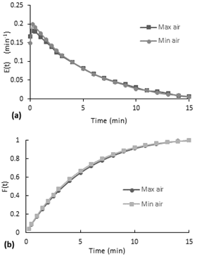
The experiment was performed with the inlet valve fully open, the reactor without the packaging mesh and with air bubble as stirring mechanism. Two tests were made with different airflow values, the first one with a minim airflow of 85 ml/s approx. and the second one with a maximum air flow of 224 ml/s approximately. The minimum airflow was defined as the flow who circulates the air through all the holes of the distributor.
Fig. 7. Residence time distribution curves for the stirred experiment without the packaging mesh.
(a) E(t) curve, (b) accumulative distribution function F(t)
According to the Figure 7-a, the E(t) curves present a decreasing behavior. At the beginning, there is a little increase to the maximum and then it starts to decrease. Although the second test is performed with almost the double of airflow, both curves have a similar behavior. (a) E(t) curve, (b) accumulative distribution function F(t)
Furthermore, the accumulative distribution (see Figure 10-b), the 60% of the dye remained less than 5 minutes in the reactor. After the injection of the dye, the flow inside the reactor acquired the same orange coloration in a few seconds (less than 20 seconds). The intensity of color decreased gradually over the time.
In a comparison of dye behavior inside the reactor between the experiments without stirring and the experiments with air stirring, is observed that in the ones without stirring takes several minutes to color all the fluid homogenously, since for air stirred experiments takes only few seconds. In addition, at the end when the last colorant comes out, for the non-stirring experiments the bottom became transparent and more orange at the top in a degrade scale, so different to the behavior of the reactor with air stirring that have the same color tone along the reactor.
3.2.2 Minimum flow, with packaging.
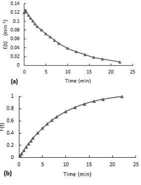
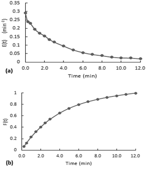
The experiment was performed with the inlet valve half open with a mean flow rate of 10.31 ml/s, the reactor with the packaging mesh and with air stirring (airflow 118,7ml/s). In this experiment is not clearly to see if there is a mixing effect of the mesh in the reactor because of the airflow while in non-stirring experiments this behavior was possible to observe.According to the Figure 8-a, the E(t) curves had also a decreasing behavior expect for the first point. As is shown on Figure 8-b, the accumulative distribution F(t) curve the 60% of the dye remained less than 7 minutes and more than 4 minutes inside the reactor.
Fig. 8. Residence time distribution curves for the stirred experiment with the packaging mesh and minimum flow.
(a) E(t) curve, (b) accumulative distribution function F(t)
(a) E(t) curve, (b) accumulative distribution function F(t)
3.2.3 Maximum flow, with packaging.
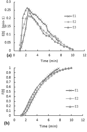
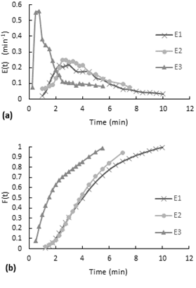
The experiment was performed with the inlet valve fully open, the reactor with the packaging mesh and air stirring (airflow 125.8ml/s). In the E(t) curve (see Figure 9-a), since the first point the curve presents a decreasing behavior. This first measurement has been taken after the injection finished. In this experiment the injection last 13 seconds, so it means that the dye gets homogenous in the reactor in less than 13 seconds.According to the accumulative distribution F(t) in the Figure 9-b, the 80% of the particles remained between 1 minute to 6 minutes inside the reactor.
Fig. 9. Residence time distribution curves for the stirred experiment with the packaging mesh and minimum flow.
(a) E(t) curve, (b) accumulative distribution function F(t)
To evaluate a flow model for air stirred experiments, is necessary to observe the behavior of the curves. According to the Figures 7, 8 and 9, all the E(t) curves had a decreasing behavior like the continuous flow stirred-tank reactor (CSTR) model, which is an ideal reactor type. For an ideal CSTR, the E(t) curve is given by the following equation (Fogler, n.d.).(a) E(t) curve, (b) accumulative distribution function F(t)
\[ E(t) = \frac{e^{-\frac{t}{\tau}}}{\tau} \hspace{1cm} (11)\] Remembering that ϴ=t/τ and E(ϴ)= τE(t) [9], then
\[ E(\theta) = e^{-\theta} \hspace{1cm} (12)\] All the experiments have a similar behavior to an ideal CSTR reactor model, but only the experiment with the packaging mesh and maximum flow starts in 1 as the model CSTR do it. In general, the experiments with the packaging mesh have the best correlation coefficient with CSTR (see table 5).
Table 5: Correlation analysis between experimental and model values of E(ϴ)
| Experiment | Correlation Coefficient with CSTR |
|---|---|
| Without mesh and min airflow | 0.971 |
| Without mesh and max airflow | 0.985 |
| Mesh and minimum flow | 0.995 |
| Mesh and maximum flow | 0.996 |
In other studies of RTD in stirred annular reactors, they also have observed in gas phase with a magnetic stirrer that a higher stirring rate broadened the RTD curve drastically and the reactor increasingly behaved as a single stirred tank reactor (Sahle-Demessie et al., 2003). Comparing a magnetic stirrer and airlift stirring, the first ones need higher velocities to produce a significant change in the RTD curve, while the second one stirs the entire flow along the reactor.
Residence time distribution (RTD) as mean residence time and variance were also evaluated, according to the equations 9 and 10. For the air stirred experiments, the minimum mean residence time corresponds to the experiment with the packaging mesh with a maximum flow operation (see table 6). Also, the lower value of variance corresponds to this experiment.
Table 6: Mean time and variance for stirred experiments
| Experiment | Mean time (min) | Variance (\(\min^2\)) |
|---|---|---|
| Without mesh and min airflow | 4.1 | 11.6 |
| Without mesh and max airflow | 4.3 | 12.2 |
| Mesh and minimum flow | 6.6 | 28.8 |
| Mesh and maximum flow | 3.5 | 9.1 |
A comparison between the experiments without the mesh, a change in the airflow does not create a big impact in mean time observed. Hence, even a minimum airflow for stirring will make a good stirring of the fluid along the entire reactor.
4. CONCLUSIONES
The pulse input experiment allowed observing the hydrodynamic behavior inside the reactor without stirring, with the presence dead zones and parallel paths. Besides, the reactor packaging is an influential factor in the movement of the particles inside the reactor, especially when working with low flows.In addition, it was determined that the residence time in the reactor without stirring comes from 4 to 10 minutes and for airlift reactor the residence time comes from 3.5 to 6.6 minutes, depending on the flow and packaging operation conditions
The analysis of the residence time distribution allowed to validate the model that best predicts the behavior of the 12-liters annular reactor without agitation. Stirred tanks in series model with n=4 fits the best for the reactor without agitation while the CSTR model is the better for the configuration of airlift reactor.
REFERENCIAS
Aparicio-Mauricio, G., Ruiz, R. S., López-Isunza, F., & Castillo-Araiza, C. O. (2017). A simple approach to describe hydrodynamics and its effect on heat and mass transport in an industrial wall-cooled fixed bed catalytic reactor: ODH of ethane on a MoVNbTeO formulation. Chemical Engineering Journal, 321, 584–599. https://doi.org/https://doi.org/10.1016/j.cej.2017.03.043Ekambara, K., Dhotre, M. T., & Joshi, J. B. (2006). CFD simulation of homogeneous reactions in turbulent pipe flows—Tubular non-catalytic reactors. Chemical Engineering Journal, 117(1), 23–29. https://doi.org/https://doi.org/10.1016/j.cej.2005.12.006
Fogler, H. S. (n.d.). Elements of chemical reaction engineering. Third edition. Upper Saddle River, N.J. : Prentice Hall PTR, [1999] ©1999. https://search.library.wisc.edu/catalog/999810177702121
Hissanaga, A. M., Padoin, N., & Paladino, E. E. (2020). Mass transfer modeling and simulation of a transient homogeneous bubbly flow in a bubble column. Chemical Engineering Science, 218, 115531. https://doi.org/https://doi.org/10.1016/j.ces.2020.115531
Levenspiel, O. (n.d.). Chemical reaction engineering. Third edition. New York : Wiley, [1999] ©1999. https://search.library.wisc.edu/catalog/999917971402121
Sahle-Demessie, E., Bekele, S., & Pillai, U. R. (2003). Residence time distribution of fluids in stirred annular photoreactor. Catalysis Today, 88(1), 61–72. https://doi.org/https://doi.org/10.1016/j.cattod.2003.08.009
Sangare, D., Bostyn, S., Moscosa-Santillan, M., & Gökalp, I. (2021). Hydrodynamics, heat transfer and kinetics reaction of CFD modeling of a batch stirred reactor under hydrothermal carbonization conditions. Energy, 219, 119635. https://doi.org/https://doi.org/10.1016/j.energy.2020.119635
Shu, S., Vidal, D., Bertrand, F., & Chaouki, J. (2019). Multiscale multiphase phenomena in bubble column reactors: A review. Renewable Energy, 141, 613–631. https://doi.org/https://doi.org/10.1016/j.renene.2019.04.020
Sozzi, D. A., & Taghipour, F. (2006). Computational and experimental study of annular photo-reactor hydrodynamics. International Journal of Heat and Fluid Flow, 27(6), 1043–1053. https://doi.org/https://doi.org/10.1016/j.ijheatfluidflow.2006.01.006
Vandewalle, L. A., Van de Vijver, R., Van Geem, K. M., & Marin, G. B. (2019). The role of mass and heat transfer in the design of novel reactors for oxidative coupling of methane. Chemical Engineering Science, 198, 268–289. https://doi.org/https://doi.org/10.1016/j.ces.2018.09.022
Universidad de Pamplona
I. I. D. T. A.
I. I. D. T. A.