Revista Colombiana de
Tecnologías de Avanzada
Tecnologías de Avanzada
Recibido: 15 de noviembre de 2022
Aceptado: 15 de febrero de 2023
Aceptado: 15 de febrero de 2023
COMPARACIÓN DE MODELOS PARA EL CÁLCULO DEL DINAGRAMA DE FONDO
COMPARISON OF THE CALCULATION MODELS FOR THE DOWNHOLE DYNAMOMETER CARD
 MSc. Jorge Enrique Meneses*, Ing. Andrea Ximena Carreño Pérez*, Ing. Sebastián Pinto López*
* Universidad Industrial de Santander (UIS), Grupo de investigación CPS.
Bucaramanga, Santander, Colombia.
Tel.: (+577) 634 4000 Ext. 2483/2829.
E-mail: jmeneses@uis.edu.co, {andrea.carreno.perez, sebastian.pinto0821}@gmail.com
COMPARISON OF THE CALCULATION MODELS FOR THE DOWNHOLE DYNAMOMETER CARD
MSc. Jorge Enrique Meneses*, Ing. Andrea Ximena Carreño Pérez*, Ing. Sebastián Pinto López*
* Universidad Industrial de Santander (UIS), Grupo de investigación CPS.
Bucaramanga, Santander, Colombia.
Tel.: (+577) 634 4000 Ext. 2483/2829.
E-mail: jmeneses@uis.edu.co, {andrea.carreno.perez, sebastian.pinto0821}@gmail.com
Cómo citar: Meneses Florez, J. E., Carreño Pérez, A. X., & Pinto López, S. (2023). COMPARACIÓN DE MODELOS PARA EL CÁLCULO DEL DINAGRAMA DE FONDO. REVISTA COLOMBIANA DE TECNOLOGIAS DE AVANZADA (RCTA), 1(41), 58–65. Recuperado a partir de https://ojs.unipamplona.edu.co/index.php/rcta/article/view/2418
Derechos de autor 2023 Revista Colombiana de Tecnologías de Avanzada (RCTA).
Esta obra está bajo una licencia internacional Creative Commons Atribución-NoComercial 4.0.

Esta obra está bajo una licencia internacional Creative Commons Atribución-NoComercial 4.0.
Abstract: The oil industry has developed the " smart well " concept to optimize production and reduce operational risk through automation. In mechanical pumping systems, it is possible to obtain in real time the "downhole dynagraph " to diagnose the system. This is achieved by using the instantaneous force and position values measured at the surface and processing them through a mathematical model called "wave equation", which represents the behavior of the rod string connecting the bottom to the surface. The accuracy of the downhole dynagraph obtained and, therefore, the certainty of the diagnoses made from it, depend on the wave equation model used. In this article, we compare the effectiveness of three mathematical models (Gibbs, Barreto Filho and Everitt) for the wave equation and by means of their solution obtain the downhole dynagraph in real conditions. The study was carried out using Python on a PC platform, evaluating the results in terms of computational performance and accuracy in detecting common operational faults.
Keywords: dynagraph, wave equation, mechanical pumping, smart well.
Resumen: La industria petrolera ha desarrollado el concepto de "pozo inteligente" para optimizar la producción y reducir el riesgo operacional a través de la automatización. En los sistemas de bombeo mecánico, es posible obtener en tiempo real el "dinagrama de fondo" para diagnosticar el sistema. Esto se logra utilizando los valores instantáneos de fuerza y posición medidos en la superficie y procesándolos mediante un modelo matemático llamado "ecuación de onda", que representa el comportamiento de la sarta de varillas que conecta el fondo con la superficie. La precisión del dinagrama de fondo obtenido y, por lo tanto, la certeza de los diagnósticos realizados a partir de él, dependen del modelo de ecuación de onda utilizado. En este artículo, se compara la efectividad de tres modelos matemáticos (Gibbs, Barreto Filho y Everitt) para la ecuación de onda y mediante su solución obtener el dinagrama de fondo en condiciones reales. El estudio se llevó a cabo utilizando Python en una plataforma PC, evaluando los resultados en términos de rendimiento computacional y precisión en la detección de fallas operacionales comunes.
Palabras clave: dinagrama, ecuación de onda, bombeo mecánico, pozo inteligente.
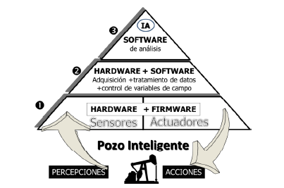
The smart well concept is based on the use of automation technologies, based on 3 fundamental pillars (Fig. 1), first: Sensors and actuators that can interact with the system, second: A hardware and software component to capture and process these variables, and third: An analysis software that can automatically generate control actions on the well.
Different multinationals offer state-of-the-art, closed and high-cost technologies that provide oil companies with the ability to obtain the background diagram, allowing them to diagnose failures during the operation process, extend the useful life of the equipment, reduce maintenance costs and increase production of the well. Colombia is a country that, as in many others, its oil wells have been in operation for more than 30 years and from which more than 50% of its reserves have been extracted; therefore, the cost associated with the acquisition of this type of high technology makes its use unattractive, given that the level of production sometimes does not allow a profit margin that justifies its purchase.
In response to this need, the Universidad Industrial de Santander (UIS) carried out the research project "8556 Prototype of an intelligent well for CEC", financed by the Vice Rector's Office for Research and Extension of the UIS, where an innovative and low-cost architecture of an intelligent well was presented (Fig. 3) consisting of two systems: one for the measurement of variables and the other for the processing of these data (Meneses y Meneses, 2020).
\[ \frac{\partial^2 y(x,t)}{\partial t^2} = v^2 \frac{\partial^2 y(x,t)}{\partial x^2} - c \frac{\partial y(x,t)}{\partial t} + g \hspace{1cm} (1)\] Gibbs proposes for equation (1), an analytical solution by applying the boundary conditions on the surface modeled by a truncated Fourier series approximation.
\[ \frac{1}{\rho} \left( E \frac{\partial^2 y}{\partial x^2}(x,t) + \eta \frac{\partial^3 y}{\partial x^2 \partial t}(x,t) \right) + g = \frac{\partial^2 y}{\partial t^2}(x,t) + \beta \frac{1}{L} \int_0^L \frac{\partial y}{\partial t}(x,t) \,dx + \gamma Q(t) \hspace{1cm} (2)\] The differential equation (2) is solved by using truncated Fourier series as Gibbs, but in this case, as the flow function Q(t) depends on the piston position values; an iterative process must be carried out until the initially estimated values of the flow converge with those calculated in the background.
\[ y_{i+1,j} = y_{i,j+1} \left(\frac{\Delta x^2}{v^2 \Delta t^2} + \frac{c\Delta x^2}{v^2 \Delta t}\right) + y_{i,j} \left(2 - \frac{2\Delta x^2}{v^2 \Delta t^2} - \frac{c\Delta x^2}{v^2 \Delta t}\right) + y_{i,j-1} \frac{\Delta x^2}{v^2 \Delta t^2} - y_{i-1,j} - \frac{g\Delta x^2}{v^2} \hspace{1cm} (3)\]
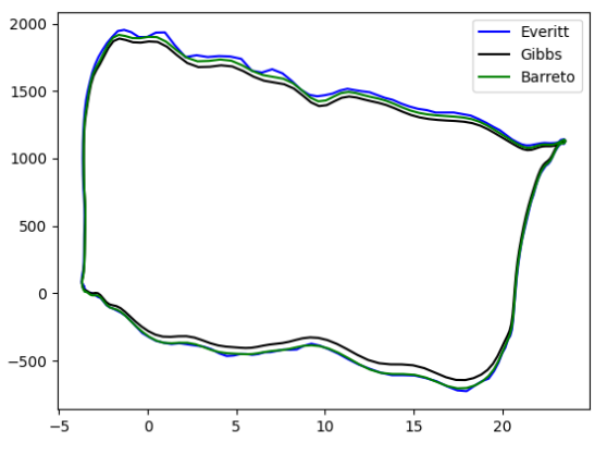
First, the software was run for the data from well 1, which has only one section. The results obtained (Fig. 5) show a very similar bottomhole dynagram among the three models, with execution times around 1 second. The model that calculated the fastest background dynagram was Gibbs, at 0.091418 seconds. The times will be presented in Table 1.

All models show effectively the same behavior; however, it is evident that the Gibbs model presents a smaller area (it overestimates friction), while on the other hand the Barreto model presents the largest area, which indicates that it assumes a much smaller friction effect than what is acting.
Again, it is evident that both Everitt's and Gibbs' models are the same, while Barreto's model still presents a background dynagram with a slightly larger area.
In addition to the evaluation of the software performance for fault detection, we proceeded to measure the execution time for each of the cases and the results obtained are shown in Table 2 below.
As in the performance analysis according to the number of sections, it was found that the Gibbs model presents a shorter execution time in relation to the other two models, and it was also evidenced that, although for most of the cases the model was accurate, for others it failed to adapt, mainly due to the use of a constant friction coefficient.
Carreño, A. y Pinto, S. (2021). Desarrollo de una herramienta software sobre plataforma embebida para la obtención del dinagrama de fondo en pozos con bombeo mecánico, Universidad industrial de Santander (UIS), Bucaramanga (Colombia). Undergraduate thesis.
Everitt, T.A y Jennings, J. (1992). An Improved Finite-Difference Calculation of Downhole Dynamometer Cards for Sucker-Rod Pumps. SPE Annual Technical Conference and Exhibition. United States: Society of Petroleum Engineers, SPE 18189.
Gabor T. (2003). Sucker-Rod Pumping Manual, Editor PennWell Books, ISBN 0-87814-899-2 PennWell Books, USA.
Garavito F. y Meneses E. (2014). Sistema Neuro-fuzzy: prospectiva de aplicación en la detección de fallas en equipos de subsuelo de unidades de levantamiento mecánico, Universidad Industrial de Santander (UIS), Bucaramanga (Colombia). Undergraduate thesis.
Gibbs, S. y Nelly, A. (1966). Computer diagnosis of down hole conditions in sucker rod pumping wells, Journal of Petroleum Technology, Vol. 18, No.1, SPE1165PA.
Gibbs, S. (2012). Rod Pumping Modern Methods of Design, Diagnosis and Surveillance. United States. ISBN 9780984966103.
Gómez A. E., Archila J.F., y Meneses, J.E. (2013). Adquisición y tratamiento de señales de un acelerómetro triaxial MEMS, para la medición del desplazamiento de una extremidad inferior, Revista Colombiana de Tecnologías de Avanzada Vol. 1, No. 21, pp. 113-118.
Meneses J.E., García J.D. y Ferreira D.A. (2015). Acelerómetros MEMS en el desarrollo de pozos y campos petroleros inteligentes, Revista Colombiana de Tecnologías de Avanzada Vol. 2, No. 26, pp. 128-135.
Meneses J.E., Niño J.D., y García F.A. (2017). KINE-UIS: modelamiento de video para la adquisición de la velocidad y aceleración angular instantánea de un sólido rígido, Revista Colombiana de Tecnologías de Avanzada Vol. 2, No. 30.
Meneses J.E., y Meneses D.P. (2020). Arquitectura Hardware/Software para un prototipo de pozo inteligente en un campo petrolero maduro, Revista Colombiana de Tecnologías de Avanzada Vol. 2, No. 36.
Meneses J.E., Garavito F.A. y Meneses E. (2021). Identificación de fallas en sistemas de bombeo mecánico de petróleo utilizando neurofuzzy, Revista Colombiana de Tecnologías de Avanzada Vol. 1, No. 37.
Sanchez J. P., Festini D. y Bel O. (2007). Beam Pumping System Optimization Through Automation, Latin American & Caribbean Petroleum Engineering Conference, Buenos Aires (Argentina), SPE 108112.
Keywords: dynagraph, wave equation, mechanical pumping, smart well.
Resumen: La industria petrolera ha desarrollado el concepto de "pozo inteligente" para optimizar la producción y reducir el riesgo operacional a través de la automatización. En los sistemas de bombeo mecánico, es posible obtener en tiempo real el "dinagrama de fondo" para diagnosticar el sistema. Esto se logra utilizando los valores instantáneos de fuerza y posición medidos en la superficie y procesándolos mediante un modelo matemático llamado "ecuación de onda", que representa el comportamiento de la sarta de varillas que conecta el fondo con la superficie. La precisión del dinagrama de fondo obtenido y, por lo tanto, la certeza de los diagnósticos realizados a partir de él, dependen del modelo de ecuación de onda utilizado. En este artículo, se compara la efectividad de tres modelos matemáticos (Gibbs, Barreto Filho y Everitt) para la ecuación de onda y mediante su solución obtener el dinagrama de fondo en condiciones reales. El estudio se llevó a cabo utilizando Python en una plataforma PC, evaluando los resultados en términos de rendimiento computacional y precisión en la detección de fallas operacionales comunes.
Palabras clave: dinagrama, ecuación de onda, bombeo mecánico, pozo inteligente.
1. INTRODUCTION
When an oil well does not have enough energy to bring the crude to the surface by itself, it is necessary to implement an artificial lift system. Worldwide, mechanical pumping (Gabor, 2003; Gibbs, 2012) is the most widely used artificial lift method, consisting of a positive displacement pump located at the bottom of the well, which is supplied with energy from an electric or internal combustion engine through the reciprocating motion of a series of connected rods (string). In recent years, the oil industry has become increasingly interested in the development of Intelligent wells and fields, because their implementation results in an autonomous, efficient and continuous operation, contributing to obtain maximum production with minimum operating costs, since it allows a quick and timely reaction to unexpected events, reducing human intervention and extending the life of the equipment.The smart well concept is based on the use of automation technologies, based on 3 fundamental pillars (Fig. 1), first: Sensors and actuators that can interact with the system, second: A hardware and software component to capture and process these variables, and third: An analysis software that can automatically generate control actions on the well.
Fig. 1. Components of a smart well.
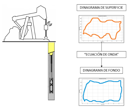
In the case of mechanical pumping, "the pump is the core of the system, and its performance has a direct impact on the economic benefit of the well and the oil field" (Sánchez et al., 2007). In the development of an intelligent oil well equipped with this type of artificial lift, permanent monitoring of the force (Meneses et al., 2015) and position (Meneses et al., 2017) values acting on the pump is fundamental, since it is the main control and diagnostic tool for the operational conditions of the system. Due to the fact that the downhole pump is located thousands of feet underground, it is obviously difficult to perform measurements directly on it, therefore, in order to monitor the performance of the system a surface dynamometer is available, which records with the rod string in motion, the numerical value of the forces acting on top of it, delivering as a result a closed curve of Force-Position called surface dynamometer.
Fig. 2. Mechanical pumping and dynagraphs.
The surface plot shows only the load applied to the downhole pump once it has propagated through the rod string and has undergone various modifications in force due to factors such as system vibrations and contact with the crude oil. Therefore, the force and position data measured at surface do not reflect the actual behavior of the downhole pump. To obtain the downhole diagram, it is necessary to mathematically model the behavior of the rod string that connects the surface with the bottom of the well, which is represented by a second order differential equation in partial derivatives, called "Wave Equation", whose solution is obtained by applying a series of mathematical processes and their corresponding boundary conditions at the top from the surface diagram (Fig. 2).Different multinationals offer state-of-the-art, closed and high-cost technologies that provide oil companies with the ability to obtain the background diagram, allowing them to diagnose failures during the operation process, extend the useful life of the equipment, reduce maintenance costs and increase production of the well. Colombia is a country that, as in many others, its oil wells have been in operation for more than 30 years and from which more than 50% of its reserves have been extracted; therefore, the cost associated with the acquisition of this type of high technology makes its use unattractive, given that the level of production sometimes does not allow a profit margin that justifies its purchase.
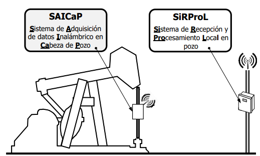
In response to this need, the Universidad Industrial de Santander (UIS) carried out the research project "8556 Prototype of an intelligent well for CEC", financed by the Vice Rector's Office for Research and Extension of the UIS, where an innovative and low-cost architecture of an intelligent well was presented (Fig. 3) consisting of two systems: one for the measurement of variables and the other for the processing of these data (Meneses y Meneses, 2020).
Fig. 3. Smart well prototype project 8556.
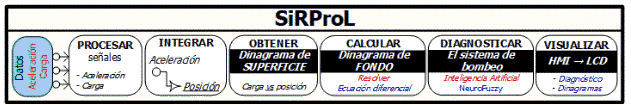
The SAICaP (Wellhead Wireless Data Acquisition System) is an intelligent embedded sensor, which instantly obtains acceleration and load data from the polished rod. Once these signals are obtained and processed, they are transmitted wirelessly to SiRProL (Local Reception and Processing System in well), which is an embedded system around a commercial motherboard, which allows to obtain in first instance the surface dynagraph, and through computational processing, to obtain the background dynagraph, for subsequent automatic diagnosis through a software tool developed (Fig. 4), based on artificial intelligence, using NEURO Fuzzy algorithms (Meneses et al., 2021).
Fig. 4. Local processing system.
Therefore, looking for an improvement to this architecture and starting from a system for data acquisition at the surface, this research focuses on comparing different models of the wave equation that allow obtaining the bottomhole dynagram in oil wells with different characteristics, thus making a comparison according to their computational performance, which will be an important variable when making decisions about which model should be implemented in an embedded system such as SiRProl, which allows the detection of faults based on the bottomhole dynagram in real time.2. MATHEMATICAL MODELS FOR THE WAVE EQUATION
The wave equation is a second order differential equation, which is derived from the application of Newton's second law and the summation of forces on a differential element of the rod string, which models the alternative motion of the rod string. Throughout history, different authors have proposed different forms for this equation, being the main difference between one model and another the way the author seeks to represent the forces generated by the interaction between the rod string, the fluid and the pipe.2.1 Gibbs
The Gibbs model (Gibbs and Nelly, 1966) is one of the most widely used models for the calculation of the bottom dynagraph. This model uses a pure viscous damping force (proportional to velocity), which is not entirely accurate since in reality the friction is a mixture between the friction generated by the contact of the string with the tubing (Coulomb) and the friction resulting from the interaction of the string with the fluid, the latter depending on the relative velocity between the string and the fluid, while the Coulomb friction is not considered dependent on the relative velocity. Even so, this dissipation coefficient, which is estimated through empirical correlations based on previous experience in the analysis of dynamometric charts, seeks to eliminate the same amount of energy that is lost through friction.\[ \frac{\partial^2 y(x,t)}{\partial t^2} = v^2 \frac{\partial^2 y(x,t)}{\partial x^2} - c \frac{\partial y(x,t)}{\partial t} + g \hspace{1cm} (1)\] Gibbs proposes for equation (1), an analytical solution by applying the boundary conditions on the surface modeled by a truncated Fourier series approximation.
2.2 Barreto Filho
Barreto (Barreto, 1993) presents a model with a more realistic formulation of the friction in the system, based on the fluid dynamic interactions in the rods and tubing, applying a model for the relative motion of a viscous fluid between two coaxial cylinders. Additionally, it does not use Hooke's law for material behavior, but instead uses the Kelvin-Voigt model for viscoelasticity, thus achieving a model applicable to wells with fiberglass rod string.\[ \frac{1}{\rho} \left( E \frac{\partial^2 y}{\partial x^2}(x,t) + \eta \frac{\partial^3 y}{\partial x^2 \partial t}(x,t) \right) + g = \frac{\partial^2 y}{\partial t^2}(x,t) + \beta \frac{1}{L} \int_0^L \frac{\partial y}{\partial t}(x,t) \,dx + \gamma Q(t) \hspace{1cm} (2)\] The differential equation (2) is solved by using truncated Fourier series as Gibbs, but in this case, as the flow function Q(t) depends on the piston position values; an iterative process must be carried out until the initially estimated values of the flow converge with those calculated in the background.
2.3 Everitt
Everitt (Everitt and Jennings, 1992) starts from the Gibbs model to give it a solution by means of the finite difference technique, but with the difference that the damping coefficient is based on the theoretical foundation of the fluid dynamic study around the string. This coefficient is determined iteratively based on the convergence between the values of the bottomhole dynamometric chart and the hydraulic power developed by the pump, thus achieving a more flexible model that adapts this coefficient to the well conditions.\[ y_{i+1,j} = y_{i,j+1} \left(\frac{\Delta x^2}{v^2 \Delta t^2} + \frac{c\Delta x^2}{v^2 \Delta t}\right) + y_{i,j} \left(2 - \frac{2\Delta x^2}{v^2 \Delta t^2} - \frac{c\Delta x^2}{v^2 \Delta t}\right) + y_{i,j-1} \frac{\Delta x^2}{v^2 \Delta t^2} - y_{i-1,j} - \frac{g\Delta x^2}{v^2} \hspace{1cm} (3)\]
3. RESULTS
3.1 Computational tool
The solution of the mathematical models mentioned above requires the use of large data matrices, such as the boundary conditions given by the surface diagram, the coefficients of the Fourier series and the values of the mesh in the solution given by finite differences. Because of this, a programming language with libraries for the treatment of vectors and matrices is required. Additionally, there must be libraries for the generation of graphics to be able to observe the background diagram and facilitate the analysis of results. With this in mind, we chose to use the Python programming language, which, in addition to meeting the requirements, is free and widely used, so that these algorithms can be implemented without financial outlay.3.2 Performance by number of sections
The performance of the software and the different models was evaluated for implementation in mechanically pumped wells with combined rod string. Therefore, the different models were evaluated with three different wells, each with a different number of sections, and then compared according to their calculation time, which was measured using the Timeit module, which is part of the standard Python library. Each program was executed ten times and the execution time was averaged. The results obtained are presented below.First, the software was run for the data from well 1, which has only one section. The results obtained (Fig. 5) show a very similar bottomhole dynagram among the three models, with execution times around 1 second. The model that calculated the fastest background dynagram was Gibbs, at 0.091418 seconds. The times will be presented in Table 1.
Fig. 5. Single rod downhole dynagram.
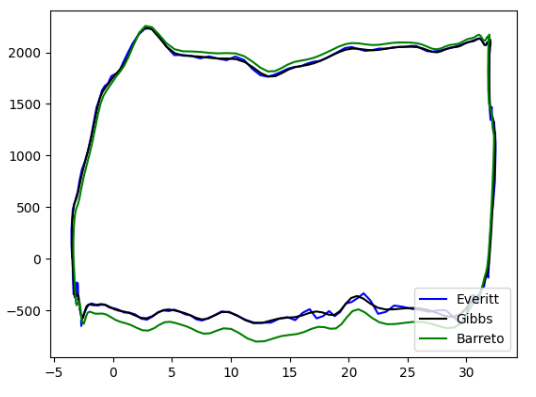
Subsequently, the bottomhole dynagram was calculated for well 2 (Fig. 6), which consisted of a combined two rod string. In this case, the execution times of the Gibbs and Everitt models increased by 23% with respect to the calculation time for a single section, while that of Barreto increased by about 78%. Gibbs was also the model with the lowest execution time, being only 0.113 seconds.
Fig. 6. Two-rod downhole dynagram.
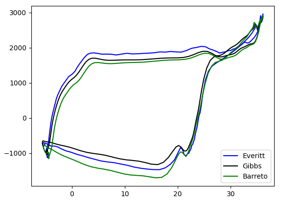
Finally, the programs were tested with the data from well 3, which had a combined rod string of three sections, for this case the calculation time increased about 10% in Everitt and Barreto with respect to the calculation for two sections, while the Gibbs model increased considerably about 57%. The downhole dynagraph obtained for the three models is shown in (Fig. 7).
Fig. 7. Three rods downhole dynagram.
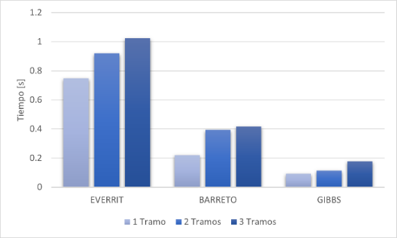
The results obtained are better illustrated in (Fig. 8), where it can be seen how the time increases for all models as the number of sections to be calculated increases. Likewise, it is evident that regardless of the number of sections the Gibbs model is the one with the fastest execution, being on average 2.7 times less than the Barreto model and even up to 7 times less than the Everitt model, which, although it solves the same differential equation, employs a numerical method for its solution. This result is quite logical, mainly because the Gibbs model is not an iterative calculation and therefore only needs to perform one run, while the other two models must perform multiple runs until the values assumed at the beginning coincide or present a minimum error with those obtained at the end of the calculation.
Fig. 8. Graph Time vs number of rods.
Table 1: Execution time according to the number of sections
| Tramos | 1 | 2 | 3 |
|---|---|---|---|
| Everitt | 0,747535 | 0,9194824 | 1,022015 |
| Barreto | 0,221069 | 0,39416178 | 0,416192 |
| Gibbs | 0,091418 | 0,11290145 | 0,177935 |
3.3 Operational failure detection software performance
The effectiveness of the different models in detecting operational failures according to the shape of the background diagram was corroborated by comparing them with the typical shapes presented in the literature.3.3.1 Gas compression
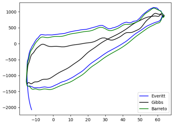
Calculating the bottomhole dynagraph for the data of well 4 and obtaining the chart shown (Fig. 9), it is evident that the net piston stroke (upper part of the graph) is much larger than the effective piston stroke (lower part of the graph), which indicates that there is gas compression since a part of the stroke is wasted producing gas instead of producing fluid, affecting considerably the pumping efficiency, coinciding with what is described in the literature about the typical form of this problem.
Fig. 9. Gas compression downhole dynagram.
As can be observed, both Everitt's and Barreto's models present a very similar behavior, on the other hand, Gibbs' model presents a chart with a smaller area, that is, less energy, therefore, it is possible to affirm that Gibbs' model may be overestimating the friction, since the friction coefficient is constant and therefore a study should be carried out to determine which would be the most accurate coefficient for the well conditions.3.3.2 Fluid Shock
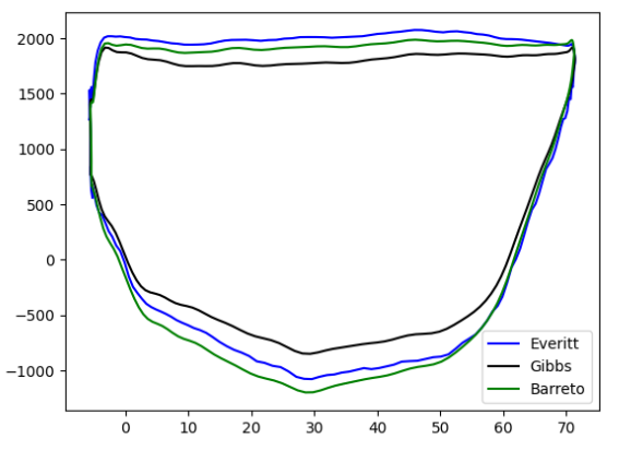
For this bottom diaphragm (Fig. 10), a difference between the net and effective piston stroke is evident, as well as an abrupt change in force, which indicates a strong fluid stroke, coinciding with the typical shape shown in the literature. Additionally, it is evident how the dynagraph is tilted to the right, which may be due to the combination of another problem, possibly an unanchored pipe.
Fig. 10. Downhole dynagram for fluid flow stroke.
It is noticeable how from the previous graph the Gibbs and Everitt models present the same behavior and areas, while the Barreto model, in spite of presenting the same shape, is slightly larger in area, which implies a lower energy loss, thus inferring a lower effect of friction.3.3.3 Leakage Fixed Valve
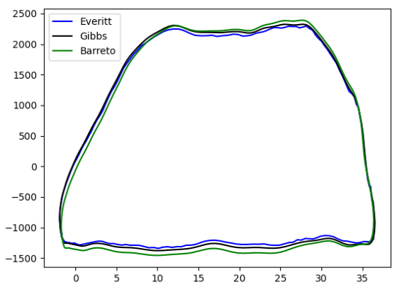
The bottomhole dynagraph obtained for well 5 (Fig.11), shows a rounding at the bottom, which according to the literature represents that there are leaks in the fixed valve because part of the fluid that is trapped in the pump is leaking back into the well.All models show effectively the same behavior; however, it is evident that the Gibbs model presents a smaller area (it overestimates friction), while on the other hand the Barreto model presents the largest area, which indicates that it assumes a much smaller friction effect than what is acting.
Fig. 11. Downhole dynagram fixed valve leakage.
3.3.4 Traveling valve leakage
The bottom dynagraph of well 6 (Fig. 12), unlike the previous dynagraph, is rounded at the top of the chart. This feature suggests a leak in the traveling valve and occurs because the valve or piston is not able to fully take the fluid load. Additionally, there is also evidence of a slight inclination to the right, which indicates that the tubing is not well anchored.
Fig. 12. Traveling valve leakage downhole dynagram.
In this case, it can be seen how almost perfectly the three models have the same downhole dynagram. 3.3.5 Non-anchored production tubing
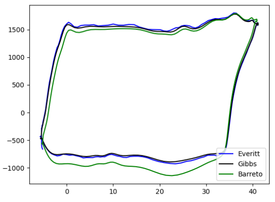
Fig. 13. Downhole Dynagram of unanchored Pipeline.
As a last case study, the bottomhole dynagram of well 1 is shown (Fig. 13), which clearly has a rightward inclination, indicating a typical bottomhole dynagram shape for an unanchored production tubing. Again, it is evident that both Everitt's and Gibbs' models are the same, while Barreto's model still presents a background dynagram with a slightly larger area.
In addition to the evaluation of the software performance for fault detection, we proceeded to measure the execution time for each of the cases and the results obtained are shown in Table 2 below.
Table 2: Failure detection performance results.
| Compresión de Gas | Golpe de Fluido | Válvula Fija | Válvula Viajera | Tubería no Anclada | |
|---|---|---|---|---|---|
| Everitt | 1,3695 | 1,4434 | 0,8589 | 0,9042 | 0,8972 |
| Barreto | 0,4687 | 0,5710 | 0,3886 | 0,3787 | 0,3437 |
| Gibbs | 0,2021 | 0,2537 | 0,1475 | 0,1407 | 0,1522 |
As in the performance analysis according to the number of sections, it was found that the Gibbs model presents a shorter execution time in relation to the other two models, and it was also evidenced that, although for most of the cases the model was accurate, for others it failed to adapt, mainly due to the use of a constant friction coefficient.
3.4 Comparison of analytical solution with an approximate solution
During this project we also developed a program that gave a solution to the Gibbs wave equation by the finite difference method, and in this way, we could compare the differences in the background dynagram when obtained by an analytical method and an approximate method, as well as evaluate its performance.
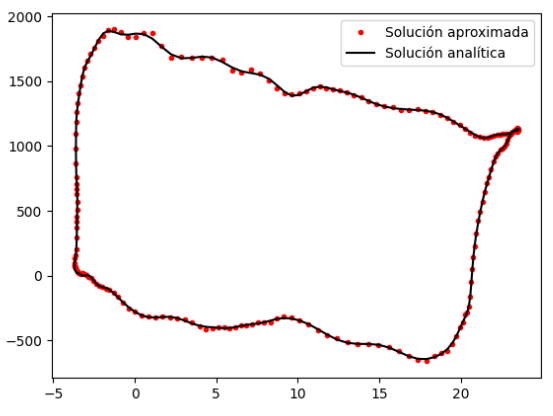
Fig. 14. Analytical vs. approximate solution
From (Fig. 14), it is evident how the two solutions obtain quite similar and accurate results at the time of obtaining the background dynagram, so the main difference between these models lies in the execution time to obtain the solution. The analytical solution takes about 0.1170 s since for this type it is only necessary to calculate the constants of each case, while by numerical methods it takes 0.2652 s, because it is necessary to perform a whole series of calculations, so that a solution by numerical methods will require more computing power.
4. CONCLUSIONS
Under the comparison of different models for obtaining the background dynagram, it was possible to conclude that the three models studied, Gibbs, Everitt and Barreto, allow obtaining the background dynagram adequately, whose calculation time increases according to the number of sections, Gibbs being the one with the shortest calculation time and Everitt the one that takes longer to obtain the solution. Additionally, it was evidenced how a solution by the finite difference method approximates very well to its respective analytical solution, however, requiring a longer calculation time (Carreño y Pinto, 2021).ACKNOWLEDGMENT
This work was part of the research project 8556 "Development of an intelligent well prototype for Campo Escuela Colorado", funded by the Vice Rector's Office for Research and Extension of the UIS (Universidad Industrial de Santander).REFERENCES
Barreto, M. (1993). Geração de carta dinamometrica de fundo para diagnostico do bombeio mecánico em poços de petróleo. Universidad Estadual de Campinas. Facultad de Ingeniería Mecánica. Masters thesis.Carreño, A. y Pinto, S. (2021). Desarrollo de una herramienta software sobre plataforma embebida para la obtención del dinagrama de fondo en pozos con bombeo mecánico, Universidad industrial de Santander (UIS), Bucaramanga (Colombia). Undergraduate thesis.
Everitt, T.A y Jennings, J. (1992). An Improved Finite-Difference Calculation of Downhole Dynamometer Cards for Sucker-Rod Pumps. SPE Annual Technical Conference and Exhibition. United States: Society of Petroleum Engineers, SPE 18189.
Gabor T. (2003). Sucker-Rod Pumping Manual, Editor PennWell Books, ISBN 0-87814-899-2 PennWell Books, USA.
Garavito F. y Meneses E. (2014). Sistema Neuro-fuzzy: prospectiva de aplicación en la detección de fallas en equipos de subsuelo de unidades de levantamiento mecánico, Universidad Industrial de Santander (UIS), Bucaramanga (Colombia). Undergraduate thesis.
Gibbs, S. y Nelly, A. (1966). Computer diagnosis of down hole conditions in sucker rod pumping wells, Journal of Petroleum Technology, Vol. 18, No.1, SPE1165PA.
Gibbs, S. (2012). Rod Pumping Modern Methods of Design, Diagnosis and Surveillance. United States. ISBN 9780984966103.
Gómez A. E., Archila J.F., y Meneses, J.E. (2013). Adquisición y tratamiento de señales de un acelerómetro triaxial MEMS, para la medición del desplazamiento de una extremidad inferior, Revista Colombiana de Tecnologías de Avanzada Vol. 1, No. 21, pp. 113-118.
Meneses J.E., García J.D. y Ferreira D.A. (2015). Acelerómetros MEMS en el desarrollo de pozos y campos petroleros inteligentes, Revista Colombiana de Tecnologías de Avanzada Vol. 2, No. 26, pp. 128-135.
Meneses J.E., Niño J.D., y García F.A. (2017). KINE-UIS: modelamiento de video para la adquisición de la velocidad y aceleración angular instantánea de un sólido rígido, Revista Colombiana de Tecnologías de Avanzada Vol. 2, No. 30.
Meneses J.E., y Meneses D.P. (2020). Arquitectura Hardware/Software para un prototipo de pozo inteligente en un campo petrolero maduro, Revista Colombiana de Tecnologías de Avanzada Vol. 2, No. 36.
Meneses J.E., Garavito F.A. y Meneses E. (2021). Identificación de fallas en sistemas de bombeo mecánico de petróleo utilizando neurofuzzy, Revista Colombiana de Tecnologías de Avanzada Vol. 1, No. 37.
Sanchez J. P., Festini D. y Bel O. (2007). Beam Pumping System Optimization Through Automation, Latin American & Caribbean Petroleum Engineering Conference, Buenos Aires (Argentina), SPE 108112.
Universidad de Pamplona
I. I. D. T. A.
I. I. D. T. A.